Bitcoin and Cryptocurrency trading is an interesting case study in emotions, especially in Envy and Greed. These are the observations as someone who never bet anything on either Bitcoin or cryptos. I haven’t written much about cryptos before, but they’re an interesting case study in the context of the emotions of Envy and Greed. Just trying to dig deep into my own head so I don’t make mistakes trading “normal” equities and options. (I personally refrained since I had no money to bet at the time, was afraid to lose, and was ramping up on options trading.)
1. Envy
Those who weren’t invested were “extremely” envious of those who made a crapload of money for no reason. It’s important to distinguish Envy vs. Greed.
Envy arises when comparing yourself to someone else, and comes from “relative” wealth. In contrast, greed is what you yourself have and is “absolute” wealth.
I’ve personally been mindful to channel any envious comparison to personal greed. These emotions are powerful and can destroy you if you don’t really understand them since they come from our evolutionary history and there’s no way to turn them off, but rather to go around them and/or channel and leverage them for useful purposes.
As a nuanced point, Jealousy is an emotion that requires both a 2nd Party, and a 3rd Party that threatens to take you already have with the 2nd Party. It’s usually involved in romantic/sexual relationships, and not usually directly related to trading/investing and economic wealth.
Greed is good. Envy is bad.
2. Greed and Fear
The ones who see others make a lot of money feel greed and want to get into crypto as well, but are too fearful to bet their own money. It’s as simple as that.
3. Crash and Self-Righteousness
Cryptocurrency and Bitcoin goes back down. Phew! The Envy has subsided a bit and the “I Told Ya So” and “They were so Dumb” statements come freely and in full force as a backwards-looking justification, vindication, and source of self-satisfaction.
4. Self-Confidence and Self-Esteem
The core here to rise above the riff raff is self-confidence and self-esteem for a healthier mind, so the following thoughts, and similar can exist instead.
– It is 100% OK that I have nothing absolutely and less relatively, since I’m happy with myself and my life.
– Those who made a crapload of money also risked a lot and could’ve lost. I did not risk anything, so therefore I have no right to be envious since I had no Skin-In-The-Game.
– I should be happy for other people’s success and try to learn from their success, rather than be envious, especially if I did not risk myself.
I’ve been doing research into all aspects of volatility to complement my options trading and VIX ETN trading.
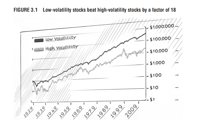
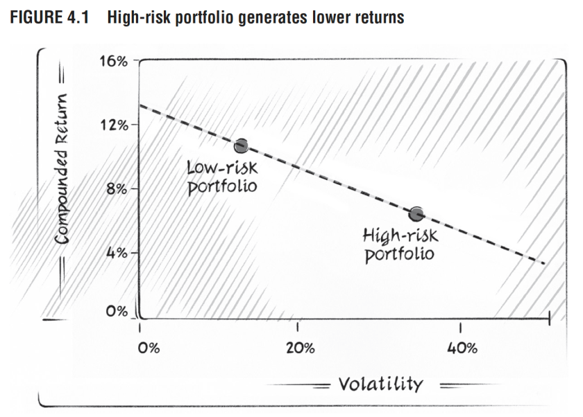
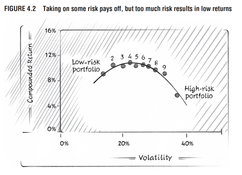
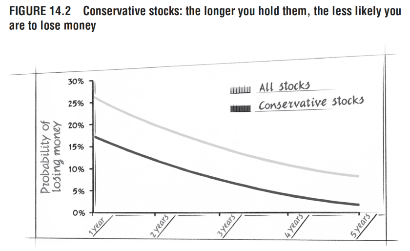
There’s a fascinating “anomaly” concerning returns being an inverse function of volatility, flying in the face of intuition and a huge theoretical edifice that returns should actually be a direct function of volatility. The framework for this was mostly built by economists and academics who spend too much time on theory and not enough time on the day-to-day profit/loss trading their own capital.
In other words, a portfolio of low volatility equities actually provide a better return than high volatility equities, since they tend to lose less during stress periods. Interestingly, this is related to how performance may be reported. Mathematically, the geometric average of return is calculated over multiple periods of time, as opposed to arithmetic averages of return calculated period-by-period. As an example, if a position loses 50% then gains 100%, then the arithmetic average return is 25%, whereas its geometric return is 0%. Talk about obscuring performance. (As an aside, this difference between arithmetic return and geometric return is at the heart of risk or money management frameworks like the Kelly Criterion, in particular, maximizing absolute portfolio growth over long periods of time using geometric averages, or about maximizing arithmetic averages over single periods of time for emotional reasons.)
Combine the framing of these returns along with fund manager compensation and fund investors benchmarks being tied to specific short periods more aligned with “arithmetic” average as opposed to multiple periods aligned with “geometric” averages, and that’s why this anomaly exists and persists in the investment industry.
This brings up two interesting philosophical issues: one concerning the nature of the relationship between related concepts of volatility, risk, and uncertainty, and the other about the human emotions of envy and greed.
These are distinct issues, but tend to be conflated together both conceptually and mathematically. I admit my definitions are not precise either.
– volatility (quantified movement)
– risk (potential for loss or bad outcomes that can be described by mean, proxied by volatility, and usually with higher moments of the distribution such as skew and kurtosis are not considered)
– uncertainty (in principle unquantifiable, but loosely proxied by statistical measures of risk like variance, skew, and kurtosis).
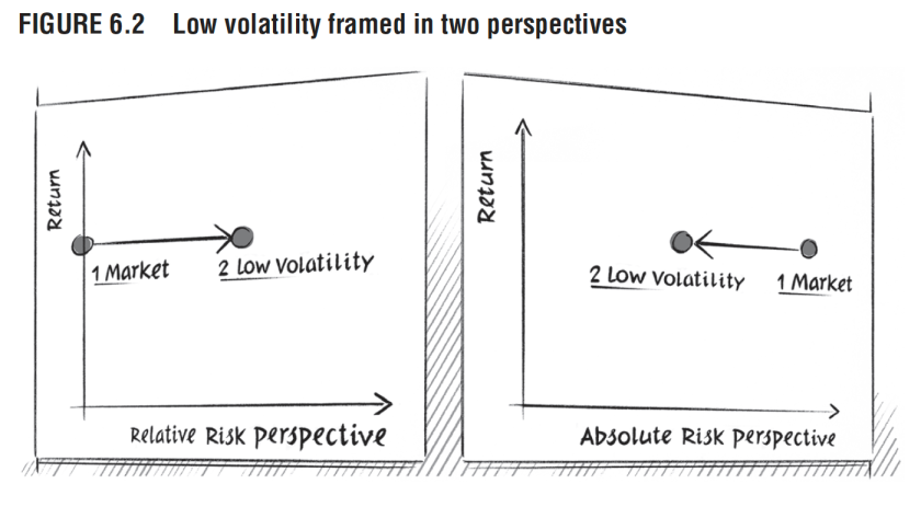
Concerning envy and greed, since fund manager performance is tied to “relative” returns to a benchmark, usually the market benchmark for their compensation and other managers for emotional and psychological reasons, instead of “absolute” returns, there’s an interesting mapping to envy and greed. Basically, “envy” arises from comparisons in terms of “relative” wealth acquisition or performance vs. greed that is more closer to “absolute” wealth acquisition and performance.
I’m trying to be as clear as I can with my thinking process towards trading and investing. Making trading decisions is an extremely emotional process in practice, even though it’s viewed as an analytical or rational process.
– Greed: Desire for “absolute” wealth that doesn’t involve other people as a benchmark.
– Envy: Desire for “relative” wealth with respect to others.
Greed is good! More specifically, striving to be Greedy and avoiding Envy is GOOD, since it allows you to to practically function very well in modern society and keep a healthy psychology to make the correct decisions. Unfortunately, Envy is the much more powerful driver.
As with all things, it makes total sense from an evolutionary perspective. Unrestricted Greed would cause (proto-)humans to maximize some utility function without context, whereas Envy is a neat heuristic to just strive to be better than average. Envy is actually more useful for both the individual and the group.
What is the emotional and personal context that I’m making a trading decision? This may be more important than the actual trading tactic or overall strategy.
Downloaded the daily closing prices of the following tickers since their inception.
NGUT/DUST, UGAZ/DGAZ, ERX/ERY, TNA/TZA, TQQQ/SQQQ, UPRO/SPXU
I chose these since they were among the most liquid, but plan to expand on the number of pairs, identity of each ticker in a pair, and or even sets of tickers on each side of the market.
2. Daily Profit/Loss
Starting from inception of the ETF and for the first day of each year for that year, backtested on a $20,000 in margin allocated to a pair, with each ticker receiving half of that, and using the daily returns based on the closing prices. This was done since inception, and starting from the first trading day of each year.
I’m assuming that this $20k is some small amount of portfolio size such as 5% – 10% so that both margin considerations aren’t an issue, and that I can short other pairs in other uncorrelated sectors. The goal is to have short pairs on five or so sectors across the entire portfolio, stressing the importance of low correlation between them. This requires more market research and backtesting, at the portfolio level one level up, which can be discussed in another (series of) post(s).
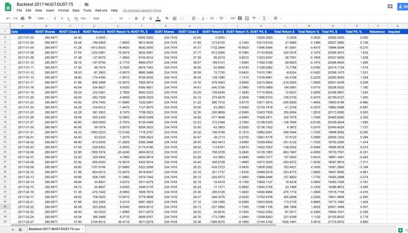
Example of a Backtest
3. Rebalancing
When shorting pairs of leveraged inverse ETFs, of course one ticker will always move up and against you. In an ideal world, both sides will eventually mean revert, and go back to the initial price you entered, minus the continuous Beta slippage losses (and other favorable losses to short positions on the underlying ETF, such as management fees), which provide the source of profit. In the real market, the side that goes up and against your position may both spike in the short term and trend in the long-term. Since shorting an ETF can lead to infinite losses, even with the mitigating factor of the winning side winning but not fast enough, one has to actively manage the allocation of the notional value of each side through a process called rebalancing.
From various posts on Seeking Alpha, it seems a crucial issue is to find the correct rebalancing threshold.
There are multiple ways to rebalance. The three classes are: A. Reduce the size of the losing side
This is useful to cut risk exposure immediately, but suffers in that it also prevents the ability to recover any losses as that losing side heads back down. B. Increase the size of the winning side
This is useful assuming we are looking at that side “only”, since we still have to account for the losses on the losing side, and those may still spike up faster than the winning side gains, depending on the the relative symmetry of the pairs. C. Redistribute the size of both the winning and losing side
Reduce the exposure on the losing side take realized profits on the winning side, and reset the trade so that they have equal exposure in terms of notional value. This is the method I used.
Example:
Let’s say I’m shorting $10k worth of $NUGT and $DUST with a rebalancing factor of 25%. The number of shares of $NUGT and $DUST would be N($NUGT) = $10k/price($NUGT) and N($DUST) = $10k/price($DUST). Now let’s say the $NUGT side moves against me and the market value of the $NUGT shares are now $13k. This would mean that I have a loss of $3k on $NUGT, and the account balance would be $7k. In a perfect world, the market value of $DUST would drop to $7k, and I’d have a $3k gain there for a total of Profit/Loss (P/L) on the pair of $0.00. In practice, I may have gained more or less than that $3k due to Beta slippage, supply/demand, management fees, etc. Let’s say I’m lucky and $DUST is showing a $4k profit so that my P/L is ($NUGT, $DUST) = ($7k, $14k), for a total $21k margin and net $1k win. What I’d do now is reset the trade by allocating $10.5k each to $NUGT and $DUST, via buying back some shares of $NUGT to reduce exposure to $10.5k and shorting more shares of $DUST to bring exposure up to $10.5k.
Of the SeekingAlpha articles I’ve read on this topic, it seems that the rebalancing percentage is crucial. In the limit that the rebalancing percentage goes to 0.0% with continuous time rebalancing, the benefits of being perfectly hedged are outweighed by transaction costs (bid-ask spread, commissions, etc) that overwhelm any wins from Beta slippage. On the other hand, in the limit that the rebalancing percentage goes to infinite (for no rebalancing), the the trade starts to become an outright shorting of the wrong side of the market, mitigated by the any the gains on the winning side.
So it’s a matter of both finding the optimal rebalancing percentage, and more crucially keeping the initial position small enough so that spikes and runs don’t cause the losing short side to be closed out from a margin call. In the backtests, I’m assuming that the position size is small enough so that it never becomes an issue. As for the rebalancing percents, currently backtesting for: 25%, 50%, 75%, 100%, 125%, 150%, 175%, and 200%.
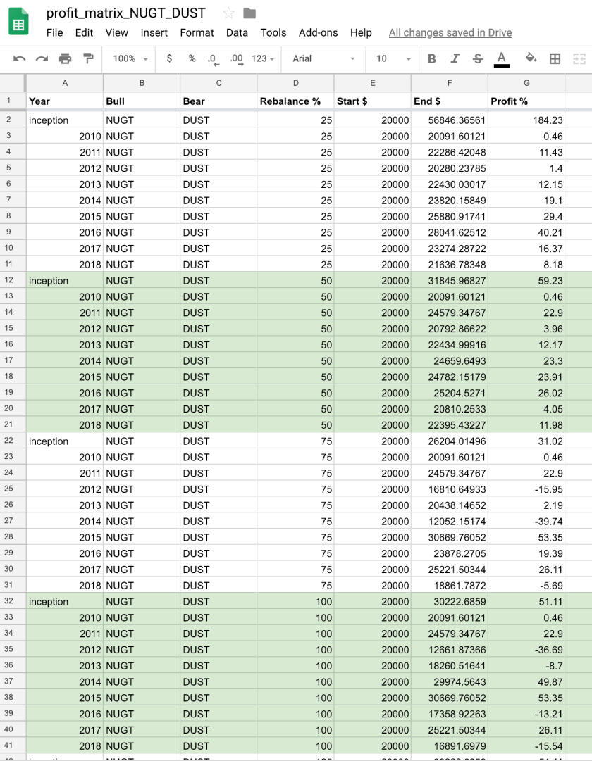
4. Results
For different starting time periods that I’m defining to be the first trading day of the year, and range of rebalancing percentages, got some first encouraging results. All of them are here in the Google Drive Folder: Backtest 1.0
Profit given different starting dates and rebalancing parameters
5. Future Work
I have much more to write with respect to limitations, improvements, and analysis, but this post is approaching 1,000 words, so will conclude now with some next action items.
Determine if there any rebalancing thresholds for each pair stand out as the most optimal, for:
Different date ranges within current tickers
Expanded ETFs
Different “paired” tickers
Write code for a portfolio of N pairs, extending beyond just one pair at a time
Model transaction costs
Bid Ask spreads
Short borrowing fees
Commissions
Write code to pull historical futures term structure to calculate contango or backwardation, and incorporate this into bias for relative weights of 3x vs. -3x ticker
To get a better feel for the decay rate of these leveraged ETFs, I was considering the following toy model with very simple assumptions.
1. Benchmark daily movements can only take: x% up, y% down
2. For trading days N, there are k up days, N-k down days
3. Leverage Factor: F
4. Composition of p% F Leveraged and (1 – p)% inverse or “-“F leverage
5. No favorable transaction costs to shorts: management fees
6. No unfavorable transaction costs to shorts: SLB interest, bid-ask spreads, etc.
Much more work to be done incorporating the following, as well as with real data, but this was a start. May want to consider the following for starters, at the risk of much greater complexity:
1. Distribution of percentage movements: d(x, t), d(y, t)
2. Multiple leverage factors F_i
3. Time dependence of leveraged and inverse: p(t), 1-p(t)
4. Representative classes of leveraged & inverse leveraged
3x SPX: SSO, UPRO, SPXL
-3x: SPX: SPXS, SPXU
I wrote a simple Python script that generated some data:
I’ve been doing research all day today. Just wanted to summarize some interesting findings.
A. Classes of ETNs
Below are charts of each pair of 3x leveraged ETNs (Exchange Traded Notes). Will only post a couple of pairs since they all pretty much look the same. I just wanted to get a high-level understanding of the pair correlations and general trends at different timeframes. In fact, the following observations are sufficiently general and may apply to classes of N times leveraged Bullish and Bearish, so the strategy is not confined to a strict matching of ETN pairs. For example, to track the S&P500, ProShares provides the 3x $UPRO and -3x $SPXU ETNs, while Direxion provides the analogous 3x $SPXL and -3x $SPXS ETNs. Due to imperfect daily tracking, management fees, and other real-world trading issues, each officially inversely-correlated pair are only inverse up to some band of variation anyways.
It seems that the utility of treating these ETNs as classes help to mitigate some problems around liquidity: bid-ask spreads and volume, both of the underlying ETNs and their options chains. Since the corresponding 3x leveraged ETNs from Direxion, VelocityShares, and/or ProShares can be substituted for each other, they effectively becomes a set of closely-related leveraged bearish/bullish ETNs that constitute an meta-ETN that may mitigate problems with liquidity in any one of the constituents.
Top row is the bullish ticker, and bottom row is the bearish ticker. Going left to right are 3 months, 3 years, and 10 years.
$NGUT vs. $DUST for 3 Months, 3 Years, and 10 Years$UGAZ vs. $DGAZ: 3 Months, 3 Years, 10 Years
– Observations
3 Month: daily inverse correlation seems very strong, as expected
3 Year: Decay of the ETNs are clearly visible
10 Year: Decay makes the last couple of years not even show up!
B. Useful Articles
Below are links to useful articles with 1 or 2 important insights
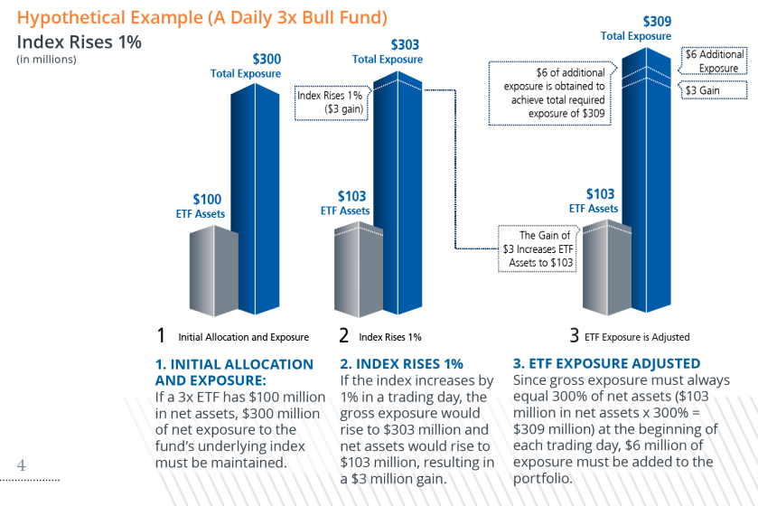
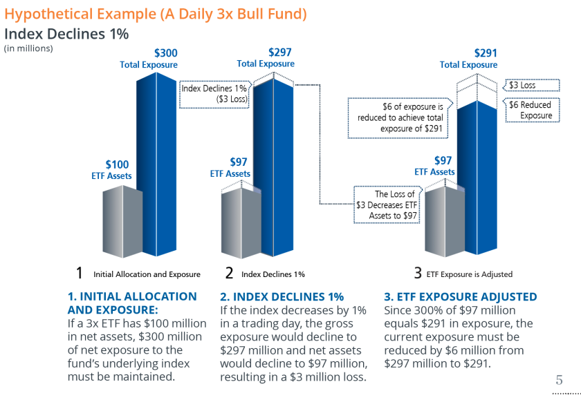
Two very good graphics showing how leveraged ETNs are rebalanced. The important thing to note here is that the very nature of the ETN construction is such that the fund is forced to “Buy High and Sell Low.” Taking a step back, this strategy would necessarily cause a loss in fund value, with the exception of a strongly trending market. And this is before any management fees are charged to the assets.
3x Leveraged Bull Fund Increase3x Leveraged ETN Decline
Takeaway: To maximize the effects of Beta slippage, choose ETNs with as low a Sharpe ratio as possible, as in having returns as close to zero and volatility as high as possible. This
Great old-ish article about this strategy, but what I really liked was the comment by a poster “Convoluted” about how shorting options may be a nicer refinement.
Comment about selling options instead of shorting underlying directly
Nice dashboard showing the decay rates of various ETN pairs. Slightly outdated since the article is 2.5 years old, and may need more ETNs pairs, but a good overview of various sectors.
Nice article that highlights practical problems of shorting the underlying leveraged ETFs, especially with respect SLB (Short Lending and Borrowing) rates. This article has convinced me to focus initially on options rather than shorting the underlying directly, whenever possible.
A bit more progress since the last blog post. In the same way that I believe long-term consistent execution will trump brilliant “ideas” or hidden “secrets”, I believe the extraordinary emerges out of the ordinary done in a consistent process-oriented way. In this trade strategy, I’m aiming for consistent forward progress. A bit more thinking to get a slightly better understanding. A bit more coding every day to build up a large trading system. A bit more every day. Relentless forward progress.
A. How is this strategy different than outright short Iron Condors?
1. Beta Slippage
Must research if Beta slippage priced into option chain, but even assuming it is, can short both underlyings directly & eventually win from twice Beta slippage (of course, assuming sufficient time & margin). Perhaps the superior modified trade is short both underlying, with long cheaper far OTM calls for protection.
2. Decay vs. Mean Reversion
ETN decay is like the underlying in condors getting pulled towards middle, may be stronger than normal mean reversion.
3. Market Efficiency
Market may price condors more efficiently due to more obvious relation on 1 underlying vs. “synthetic” 2 underlying position.
4. To Investigate
Directly shorting 2 anticorrelated underlyings
Short options spreads on them
Short underlying with long cheaper far OTM for large protection
This may involve research into the liquidity of underlying and options chain for the bid-ask spread & volume, higher moments of the option chain in time and strike, frequency and size of moves.
B. Connection to PostgresSQL
Data from the Interactive Brokers API dumped to spreadsheets and uploaded to the Google Drive Folder: Infinite Decay are nice for initial data exploration and visualization, and are very useful to share with anyone I interact with, but more intense data ingestion (scrubbing, transforming, updating, staging, etc.), read/write operations, backtesting and analysis, and algorithm development will require a much more functional data management system. I’ve decided to use PostgresSQL (PG) as my database for data operations.
SQL scripts to create database tables for use for the ticker data and paired ticker data
Connection to PG in Python using the most popular psycopg2 adapter
The code references a local instance of a PG database, but it can very easily be adapted to a cloud hosted instance by simplying changing the host in the psycopg2.connect( ) function
Preliminary functions to load the tables with the data from the IB API and CSVs
Will write more general CRUD functions in a database worker class, just wanted to finish off making the first connections
Tech commentary: I like the feel of SQL queries better than NoSQL, since the query language is very expressive and lightweight. Technically and information theory-wise, it’s of course possible to use either and to replicate one in the other. What’s really cool is that PG has a data type called “json”, which allows storage of JSONs to emulate NoSQL. This is extremely useful to combine the expressiveness of SQL with the universality of JSON, for example, can build API endpoints using JSON with minimal effort and the open source search engine Solr is effectively a JSON / NoSQL content management system.
I’ve decided “Infinite Decay” would be a good name for the trade strategy outlined in the previous blog post about shorting bear call spreads on inversely-correlated leveraged ETFs to take advantage of the following:
Underlying: Beta slippage of leveraged ETFs
Underlying: Decay from futures roll yield
Negative correlation of ETFs (neutral underlying neutral exposure)
Options: Theta decay
Options: Implied Volatility premium
This post will outline preliminary work I’ve completed with some comments regarding technical, trading, or financial aspects, and tangible next steps to pursue.
A. Completed: Preliminary Data for Tickers
Wrote a bit of Python code (Git Repo below) to connect to the Interactive Brokers API to pull down closing data for the preliminary Exchange Traded Notes (ETNs) to investigate.
Gold: $NUGT / $DUST
Natural Gas: $UGAZ / $DGAZ
Energy: $ERX / $ERY
Small Cap: $TNA / $TZA
NASDAQ: $TQQQ / $SQQQ
SP500: $UPRO / $SPXU
Comparison of $NUGT vs. $DUST
Data
Data goes back to the start of these tickers, but will need to take various slices to reflect market and macroeconomic regimes
Missing Data
A bit of processing needed to process the data stream from the IB API since some dates were missing. Missing entries were filled with the closing prices of the previous close, with percent gain set to zero
Index
The “Index” column starts at an arbitrary 1,000,000 on the first day of data to simulate an outright long position. Can adjust accordingly
Google Docs
I’ve uploaded into the Folder: Infinite Decay the following:
– Raw data files from IB with the ticker names
– Processed versions combining the pairs: Pair – < Bull Ticker > & < Bear Ticker >
B. Open Source Code
I’ve decided to open source as much of my code as possible so that I can be as useful as possible to anyone I interact with. I take the view that there are no real lasting secrets ideas in the markets and that long-term consistent profitability is ~100% execution. Even if you can somehow emulate execution blindly with all secrets at a certain point in time, the markets continuously evolve so much that your ideas, trade strategies, and code will need to be updated anyways. Essentially, it’s not first-order competence as in what your trade strategy is or what code you wrote, but second-order competence at how well you can adapt the strategy and write better code, and even third-order competence as in how “fast” you can iterate and improve.
Python Code
It provides working Python code to connect to the Interactive Brokers API, which works with either TraderWorkstation and/or IB Gateway clients. Much more to write here that could involve a series of blog posts. Beyond the scope of this post, but I might write some tutorials if requested, along with more documentation of the code.
Preliminary Uses
Main function: Downloads historical tick data given various parameters such as functions, time frames, etc. for the leveraged ETF tickers above, along with code that processes and normalizes that data to be uploaded to the Google Doc Folder: Infinite Decay
C. Immediate Next Steps
Research ETN Fundamentals
Compile larger list of inversely correlated tickers and skim all the prospectuses of Exchange Traded Notes, for example, $UGAZ / $DGAZ to see if there’s any hidden bombs I should be worried about
Additional Ticker and Options Data
Download and normalize relevant ticker and associated options data such: volume (important!), daily implied volatility, and historical volatility for the tickers above and rank in terms of liquidity.
Specific Market Understanding
General reading of the markets and futures markets of the commodity or area that these ETNs and futures track
People and Blogs
Start following traders in this general strategy and/or these markets, and compile list of blogs or articles.
D. Additional Thoughts
My initial thinking on this particular strategy involves symmetrical options spreads to take advantage of the decay, but was also thinking of further improvements. Will need to be very open-minded in related strategies to adapt to market conditions
For example, take an outright short position in the underlying while buying cheap and long far out of the money options position as a cheap hedge. This might be necessary if the options markets are not very liquid, in terms of large bid-ask spreads or low volume or open interest.
Don’t count out the possibility of temporarily modifying the trade if given a very strong reason, such as a large market shock, either via biasing the trade one way or taking an outright uncovered long position Bullish or Bearish the market.
Trade Idea: Short bear call spreads on paired 3x leveraged & “inverse” 3x leveraged ETFs (ETN, ETP) to benefit from decay of underlying and options
Some preliminary thoughts of a trade idea before diving into more detailed research.
A. Core Rationales
1. Underlying: Beta slippage of leveraged ETFs
2. Underlying: Decay from futures roll yield
3. Negative correlation of ETFs (neutral underlying neutral exposure)
4. Options: Theta decay
5. Options: Implied Volatility premium
B. Risks
1. Sustained multi-day runs that amplify leverage of ETFs
2. Exercise of options for underlying
3. “Missing out” on strong directional trend on either side
C. Mitigation
1. Option spreads
2. Can convert exercised options to short underlying (potentially with long options for hedge)
3. Small position size: 3%-10% of portfolio
4. Rebalancing: after X% rise in underlying, exit and reset
D. Considerations
1. How anti-correlated are the underlyings?
2. Need small enough position for (almost) inevitable win, but not small enough WRT transaction costs
3. Wider options spread widths to limit number of spreads (lower transaction costs & bid-ask cross) 4. Short option strike closer to ATM to maximize short extrinsic value
E. Further Research
1. Liquidity(!): Create ranked list of most liquid underlyings and most liquid options chains
2. Average Beta slippage for each pair
3. Average Decay for each pair
4. Intraday and multiday spikes and runs: get worst, average, and median
5. Simulation/Backtest: Daily % & dollar moves of underlying
From the small sample size of the ongoing trade of short options on $VXX, I believe I can maintain a ~100% return on invested capital. To take a current trade as an example, $45k margin collateral is scheduled to net me $10k over 2.5-3.0 months, or between $40k and $48k per year. This is assuming constant margin collateral of $45k and no reinvestment of capital, which of course could boost this a amount significantly, but I’m focusing only on the per-trade return, not on the entire portfolio. If I can cycle through about four of these trades per year, it would be the ideal, ongoing, core focus of the options strategy.
Can I do better to get better return and with less risk?
I believe so. So additionally, I’m researching how to boost return even more by pursuing earnings trades in between these 4x core trades that last 2.5-3.0 month each. The basic idea behind earnings trades is that options become highly over-inflated in price leading up to earnings. Once earnings figures are announced, options may rapidly lose value in the collapse of implied volatility in a “single day” what it might take them 1-3 months to lose in non-earnings contexts.
Similar to $VXX, it’s possible to go long options (long implied volatility, aka: long IV). In this case it would be to go long IV leading up to earnings announcements. However, research I’ve done shows it’s very hard to time the increasing options IV, so my strategy instead is to short IV right before earnings, and exiting within one trading session.
To summarize, my plan for opportunistic earnings trades:
1. Research what underlying stock has historically the greatest drops in implied volatility at earnings announcements, preferably accompanied by the least movement in stock price
2. Commit 1%-5% of margin capital per earnings trade during earnings seasons, in between the core $VXX trades, to short straddles/flies and/or strangles/condors for 1-day trades
3. Automate this process via Python code connecting to the Interactive Brokers API to to hit 60 earnings trades per quarter for the most highly liquid options on the most highly liquid underlying stock