Seeing how Coinbase.com and some other crypto exchanges are now having massive trouble processing transactions and even a total inability to login, it brings up to the forefront the primacy of market liquidity as the single most important risk management issue and trading strategy consideration.
Coarsely put, liquidity is that feature of markets that permits easy entry and exit at relatively stable prices. I really believe liquidity will be “the” determining factor in how Bitcoin and other cryptos evolve in the immediate next few days as the exchanges get overburdened and there’s a crazy rush to the same “illiquid” door out, and long term as prices stabilize a bit.
Interestingly, liquidity and “flight to quality” to US treasuries was the one issue that the two Nobel Laureates: Robert Merton and Myron Scholes, did not account for when their multi-billion dollar hedge fund Long Term Capital Management blew up in the 1998 when Russia defaulted on its bonds, sucking up the liquidity of the markets in which they held their multi billion dollar positions, ultimately causing that hedge fund to implode in spectacular fashion with the Fed and multiple Wall Street banks getting involved, LOL! It’s all detailed in Roger Lowenstein’s “When Genius Failed.” If Merton/Scholes’ models worked in the real world as they did in academic theory, those two would be billionaires multiple times over now.
Thinking about strategies in general, especially WRT to the voodoo/astrology known as Technical Analysis (to be fair, TA is not 100% BS since it can be a self-fulfilling prophecy as everyone sees the same price action and patterns, so maybe only like 90% BS – I think of TA as applied groupthink or social psychology), any stop losses or take profit targets, any entries or exit strategies, transaction cost analysis, and so on are actually issues of liquidity.
I’m finding that over 80% of my time in coding up my options trading platform is dealing with liquidity, in the sense of finding tight bid/ask spreads, volume for options, open interest (current outstanding options contracts), and liquidity of the underlying security, mainly stocks, but can be futures, currencies, bonds, ETFs, and so on). Liquidity may be the fact that turns a medium-quality winner into a loser, or a big winner into a tiny winner, or a tiny loser into a huge loser.
I take the view that long-term persistent profitability in discretionary trading strategies is impossible because the trader must repeatedly get all three of the following factors correct: Direction, Magnitude, and Speed. This post was written primarily with stocks in mind as the particular asset class, but these ideas can apply to other asset classes such as futures, bonds, currencies, etc. or “buying” options, where profit and loss result from a buy or sell decision tied to the future direction of the security. The counterexamples will involve the “selling” of options.
One way I conceptualize the market is in terms of states of the universe, and attempting to explicitly pick a particular smaller set of states in that entire universe is much harder than being agnostic and implicitly picking a larger number of states. Let’s consider Direction, Magnitude, and Speed in turn.
Direction
It’s hard or even impossible to pick the direction of price movement, which is effectively random. (Paradoxically, it’s this random and unpredictable nature that permitted the entire mathematical structure modeling price movement via such ideas as Brownian motion.) Let’s assume there are three states of price action:
up
down
flat
Discretionary trading or buying options would require that you correctly pick 1 of 3 states correctly, whereas in contrast an options selling strategy would just require that you did not fall into that one particular category. So in effect, you can be “correct” 2 of 3 times by avoiding being “incorrect” only 1 of 3 times.
Magnitude
Assuming you can correctly pick the direction of price movement, then there would need to be a large magnitude move in that direction to be profitable for that thesis to be correct. Alternatively, you can have a larger amount of capital tied to a smaller magnitude move, but that would introduce commensurately larger amounts of risk. Let’s assign magnitude to two states:
small
large
There is a much larger frequency of small moves in the market compared to large moves, so trading in a security directly would mean you’d want a large move, that would be relatively smaller proportion of the entire set of states.
Speed
Assuming both the direction and magnitude of price are picked correctly, the speed at which they are realized needs to be sufficiently fast such that rate of return on investment is high enough to beat other allocations of capital, with the baseline being the risk-free rate of US treasuries. Even if a decision in correct, it may be incorrect when tied to and judged upon economic metrics. Let’s assign speed to two states:
slow
fast
So in taking a direct position in a security (or “buying” an option), you not only need to get the direction and magnitude correct, but the decision must turn out to be correct quickly enough for practical reasons. There are more states of the world where price moves slowly, rather than quickly.
Because of these reasons involving the joint correctness of direction, magnitude, and speed, discretionary trading is very difficult and in my view, effectively impossible. Therefore, a strategy which requires correctness in a narrower and infrequent way is inferior to another strategy that requires only that you are not incorrect in a broad way involving more states of the world. In other words, it’s a better bet to bet on the greater number of possible states of the universe, by explicitly not picking a smaller number of states out of an entire universe of states, to implicitly pick the larger number of states.
The practical implementation of this view is the “selling” of options.
This post is an example of the bread-and-butter operation of how panning for gold looks like in terms of the implied volatility premium in the options markets. 🙂
Panning for gold used to look like this, now it is in terms of code and data.
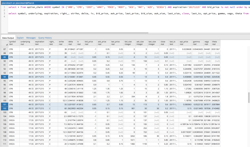
The first pic below is the relevant market data for the most important options for one of the best candidate stock examples for the Campbell Soup Company, ticker $CPB. I’ll be easily surpassing 1 million of these rows soon and the task at hand now is to sift through them much like you sift through dirt/sediment to get gold. The last pic is just a typical streaming console printout of how the raw data looks like. This stock $CPB has an implied volatility rank of 100%, meaning that its options are at an all-time over-priced high, one of the best out of the universe of 1000s of underlying stock and ETFs using the Black-Scholes pricing model.
There’s an entire discussion on implied volatility rank as the criteria for what constitutes good candidate stocks and ETFs and the finer points of scanning that and cleaning the data, but I wanted to focus on this particular tangible example of candidate spread entry.
A specific entry. Potentially many millions of such rows to sift through.
1. The rows 89, 94, 101, 102 in blue highlight the four legs of the option spread I’m considering.
2. I’ve chosen them according to the column “delta” of closest to 0.15, which is approximately the probability of the option being in the money. Choosing delta = 0.15 on both sides is picking a forward looking probability of winning of about 70%, assuming these option are untouched until expiration. Various trade adjustments can make this winning percentage go up to even 80%-90%. There’s an entire discussion about the optimal triggers to close out a trade pre-expiration, but the main takeaway is to do this more often in a dynamic optimization of recycling capital vs. decrease in implied volatility vs. time decay.
3. This is used to filter for the inner leg options on row 94 at 45 strike Put and row 101 at 55 strike Calls. Here, I can sell at the Asking price at $0.55 for the 45 Put and $0.70 for the 55 Call. This would be a net credit of $1.25 = $0.70 + $0.55. Since the multiplier is 100, I’ll be intaking a credit of $125.
3. In order to protect myself against a huge market move, I’m buying the cheaper options further out of the money at the Ask: 40 Puts on row 89 for $0.15 and 60 Calls on row 102 for $0.15. Likewise multiplying this by 100 means it’ll cost $30 combined.
4. The net credit I’m taking in therefore on this position is $95 = $125 – $30.
5. This is reduced by transaction costs of $2.80 = 4 x $0.70 through Interactive Brokers. Let’s just say $3. Compare this to TD Ameritrae that charges $6.95 base commission with $0.75/contract for a $9.95 cost for this same trade. Pretty much robbery, and may make this trading strategy unprofitable. Let’s just say $3. So the net credit I’m taking in $92 = $95 – $3.
6. My exit once the value of this spread I sold drops to approximately half, or about $45. So essentially over the course of nexgt month, I’d like to make $45 off this single position.
This is first order-approximation of one single basic position. There are effectively an infinite number of tweaks for optimization , but this basic strategy shown here constitutes 80%-90% of an entry.
Other posts will delve into these optimizations such as the following 10, which are only a subset of other considerations.
Accounting for vertical volatility skew (different strike prices)
Accounting for horizontal volatility skew (differerent expiration months)
Trade adjustments (frequency and transaction cost analysis)
The directional spread version with 30 delta to a single side, as opposed to this non-directional versionf 15 delta to each side
Liquidity in terms of bid-ask spread
Liquidity in terms of volume
Adjustment and exit criteria
Higher moments for a specific partial derivatives in the underlying (gamma, second order in underlying price) and external factors (charm, exprssing the time change of delta)
Secific earnings events
General market sentiment
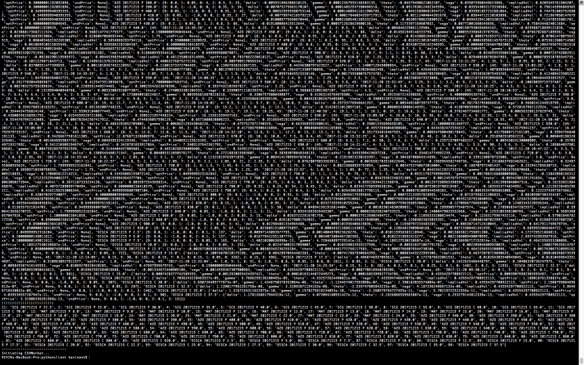
An example console printout of the data used to populate the PG SQL table.
Yet another demonstration that market efficiency stating prices in the market adjust instantaneously to reflect true value is such an absurd view invented by those who never operated in the markets.
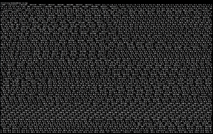
Witness this data and combinatorial explosion. This is a printout (view in full screen) of the “identities” of a small fraction of the options I’m scanning.
A small sample of strike prices and expiration dates of the highest implied volatility rank options for S&P500 stocks ending before 2018.
For each of the ticker prices here, the number of expirations listed here multiplied by the strike prices, which is then multiplied by a Put and Call. This is one of many screen of the expirations and strike prices of the next month of stocks in the S&P500 with implied volatility rank of greater than 60th percentile expiring in 2017. If you include all of 2018 options and include bid/ask prices and bid/ask volumes, updated in “real time”, this data increases orders of magnitude more.
Market efficiency would mean that the true values of these associated bids and asks tied to a every single one of these option expirations and strikes would get updated in real time such that there are no opportunities to benefit from mispricings. Just ridiculous and even physically impossible, forget about financially impossible.
Assuming every market participant had a supercomputer with infinite processing power and transaction costs were precisely $0.00, you’d “STILL” encounter speed-of-light issues in information transmission.
In fact, I’d say it’s a physical limit you’re hitting precluding market efficiency.
An important component of my options trading system is to scan securities in the market and order them by the Implied Volatility (IV) rank of the at the money options tied to the candidate underlying securities for which to sell options for. In theory this is straightforward, but in practice, there are many higher-order modeling and execution issues when practically implementing software, accounting for the messy nature of data, and navigating market microstructure. This post will start with more specific, technical, and practical issues before considering more these higher order issues, and then ultimately why some can be ignored.
The first table below are from a universe of securities comprising the S&P500 and the top 10 ETFs with most liquid options such as $SPY, $EEM, $QQQ, and $IWM. The data obtained was represented in terms of bar data (high, low, open, close) for implied volatility. In the tables, the date is today’s date and not expiration. The iv_rank is a simple calculation with potentially non-trivial assumptions.
Highest Implied Volatility Rank S&P500 stocks as of Nov 5, 2017Lowest Implied Volatility Rank S&P500 stocks as of Nov 05, 2917
Some modeling assumptions, with some commentary or questions:
Timescales: Lookback period is T(lookback) = 1 year and unit is T(unit) = 1 day
How does this change with different configurations of T(lookback) and T(unit)?
Bar Data: Historical data was obtained in terms of bars with (high, low, open, close), and I used the midpoint of the open and close bars.
How would this change if using: (a) close only, (b) midpoint of high and low, (c) average of high, low, open, close
Outliers: No outlier handling done
For future versions, I may want to remove top N outliers points so that the IV rank is unaffected
Precision of Data: Need to corroborate this with multiple sources
May not actually matter since the main relevant issue is whether the IV rank is high vs. average vs. low. Even getting a few percentile points wrong in the IV or IV rank may not be relevant
Furthermore, there are more considerations when actually executing the trade
Liquidity
This may actually be equivalent to enough IV and IV_rank percentages worth if not accounted for, making a very favorable trade into a neutral or even non-favorable one. Currently using a benchmark of 500 Contracts worth of open interest of at the money options, with a volume of 2000. Will need to analyze this but it falls within the parameters of a decent set
Transaction Costs (see [*] below at end of post)
The nature and cheapness of the transaction cost structure through Interactive Brokers, as well as my pursuit of automated decisions, is such that I’m not penalized and actually incentivized to do more frequent adjustments. This implies I should try to maximize the quality of data obtained, analysis depth, and precision of trading decision should.
Vertical Skew
Will need to study the IV, and perhaps IV rank skew, of the options chain as a function of strike price and underlying price tied to each of these particular high IV rank securities to see to what extent I should make proper adjustments for entry, managing, and exit.
Horizontal Skew
Same as considerations in vertical skew, but in time, as in horizontal skew
Days until Expiration Theta (time decay) grows in an accelerating fashion benefiting a net seller, whereas gamma risk increases as well.
Ultimately, to what extent should I worry about these higher order modeling and execution issues? I suspect that this may rapidly become an issue of excessive or false precision relative to the core tenets of my strategy outlined below that may actually be vastly more important, until I scale up in number of positions and/or size of positions.
Small positions per trade
In order to limit idiosyncratic risk tied to a specific security or event
Scaled to an infinite number of trials
To permit probabilities to work out
High probability of success
I’m targeting a probability of winning of 70%, roughly corresponding to a movement of one standard deviation at 68%.
This is practically implemented by targeting options spreads with a Delta of 30 on one side for single vertical call or put spreads, or two call/put spreads (Iron Condor) for a Delta of 15 on either side.
Liquidity
As stated above, a relative lack of liquidity may actually be worth much greater precision’s worth of modeling and execution realties.
Net Selling Strategies
To capture the IV premium
Benefit from Theta time decay
There are cases where a net buying position may be favorable, such as in an extremely low IV rank environment
Assuming that I stick with these fundamentals, high-order modifications may only start to matter at much greater volume or position scales. It reminds me of the situation in No Limit Texas Hold’em poker where one could refine their “trading” strategy by incorporating the finer points of Game Theory, the probabilities of for all situations, model opponent tendencies according to physical tells and psychological profiles, and so on. Alternatively, one could just stick with two important rules that actually have very little to do with the specific modeling or execution:
Play more hands in later position
Play bigger pots with bigger hands
Adding more complexity is easy, removing it and distilling only the essence of a strategy so that it’s robust for many contexts and provides a great margin of error may be the more difficult thing to do. In my case, more complexity may entail more complex options pricing model, more data, better software, more contingencies to account for. More simplicity may entail a few core powerful principles that reduce
[*] Commentary: Transaction costs
A huge issue here is transaction costs.
Interactive Brokers (IB) charges $0.00 base fee and $0.70 per contract. Compared to getting totally crushed by TDAmeritrade (TDA) $6.95 base fee and $0.75 per contract.
1. One contract case
IB: $1.00 = max($1.00, $0.70) (since the smallest commision charged is $1.00)
TDA: $7.70 = $6.95 + $0.75
For a single market-neutral risk defined spread with 4 single positions that consitute a Put Credit spread and a Call Credit sprad, it would cost $2.80 with IB and $9.95 with TDA. This is a clear advantage with IB, but it gets even better for adjustments to manage a side of a trade that may only touch 1 or 2 positions, in which case, the base fee difference of for IB at $0.00 vs. TDA at $6.95 becomes an even bigger issue.
What constitutes a good bet in theory and in practice? How do psychological and emotional states affect what constitutes a good bet? In this post, I explore the tension between subjective psychological states and objective mathematical expectation. It’s important to lay out the assumptions behind expectation that are usually taken as axiomatic and viewed as the correct way to make decisionsk versus how they actually affect real-life decision-making.
Classical economic, financial, and gambling theory states that making a bet should only be dictated by the expectation of outcomes of the bet. Let us consider the following:
X = Expected Payoff
p(win) = probability of winning bet
X(win) = payoff of winning bet
p(lose) = probability of losing bet
X(lose) = payoff of losing bet
X(total) = p(win) * X(win) + p(lose) * X(lose)
The assumption is that any bet (ignoring transaction costs) with
X(total) > 0 is a good bet and should be taken
X(total) < 0 is a bad bet and should be avoided
X(total) = 0 is a neutral bet and should be viewed with indifference
Indeed these are great assumptions, but they’re only a start. There are other issues involved such as the shape of the underlying distributions and payoffs, in particular:
What are the relative sizes of the probabilities: p(win) and p(lose)?
Are they similar such that p(win) = p(lose) = 50% resembling a coin toss?
Are they vastly different such that p(win) << p(loss) resembling a lottery ticket?
Are they vastly different such that p(win) >> p(loss) much like an seller of insurance wins?
What are the relative payoffs: X(win) and X(lose)?
Are they similar such that X(win) = X(lose) resembling a fair coin toss?
Are they vastly different such that X(win) >> X(loss) resembling a lottery ticket?
Are they vastly different such that X(win) << X(loss) much like collecting the premium of as a catastrophic insurance writer?
How is the total expectation X realized?
Similar size wins and losses?
Much larger wins than losses like in a lottery?
Much larger losses than wins like a seller of insurance?
As the number of bets goes to infinity and the “ability” to take those bets is infinite, it actually doesn’t matter too much since positive expectation will work itself out for a net gain despite any short term variance that can bankrupt you. Practically, however, things are much different since you can go bankrupt and have no more betting capital, and your emotional state may cause you to choose or at least prefer suboptimal outcomes.
According to Prospect Theory:
People much prefer to avoid loss of any kind and are willing to take much bigger risks when down to get back to even
People much prefer to lock in gains, and are willing to take much smaller risks when up to lock in the gains
This most likely comes from our evolutionary history in that it’s not mathematical expectation that’s being maximized for in a Platonic context , but rather optimization of expectation of survival simply to survive in the context of very limited time and information processing. What implications that this have for trading and risk taking?
If we introduce utility functions that assign a value to both the probabilities and payoffs of winning, losing, and their total expectation, it may help us to better understand. Introducing U(x) as the utility of X, we now have the expectation equation as:
I would say that the main components of this equation that people actually care about are:
Maximizing U[p(win)]
Which means that people prefer to win with higher probability with related higher frequency above all else
Minimizing U[p(lose)]
Which means that people prefer to lose with lower probability with related lower frequency above all else
Preference for U[p(win)] >> U[p(lose)]
Even if this means a lower expectation
From my observations of my own preferences and emotional state, as well as other people’s in any betting or risk-reward context, whether it’s at a poker table or trading in the markets, this appears to be true more true than not. This has many implications for trading and betting strategies, which I’ll explore in later blog posts.