Volatility Skew and Prospect Theory

A fundamental tenet of options trading is the capture of as much implied volatility (IV) premium as possible as a net sellers of options in a high IV context. To refine my trade entries, management, and exits, I’ve been doing a bit of research to better under backwards-looking, historical, statistical data in order to formulate forwards-looking, predictive, probabilistic trading.

(Note: It’s important to distinguish between these two since they’re often conflated. In grad school,  I had a debate that power laws describing severity vs. frequency of events are descriptive statistical empirical facts and just NOT be confused with predictive and probabilistic in theoretical models.) 

One strange phenomenon is the shape of IV as a function of strike price for the same-expiration options across the option chain.  Black-Scholes predicts a flat shape, but what we encounter are  as we move away from at-the-money (ATM) options to out-of-them-money options is an upward sloping graph.

Implied volatility smile

Furthermore, there tends to be a skew to this graph such that lower OTM Put strike prices tend to have greater IV than higher OTM Call strike prices.

Implied volatility skew

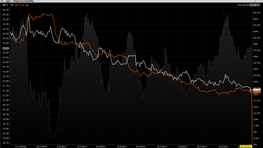
Indeed, we see this in the real world as well.

Volatility Skew in a real-life example: SPX Options

The main related questions I have are:

• Why are out of the money options increasingly more expensive?
• Why are out-of-the-money OTM Puts more expensive than OTM Calls?

It would appear that there are two distinct reasons underlying both of these phenomena that make sense.

Reason: Higher uncertainty further away from strike price

Options pricing models are obviously not terrain, but only a map of the terrain with many simplifying assumptions and parameters that may render the model decreasingly with increasing uncertainty. This diminished usefulness and greater uncertainty manifests itself as an increasingly larger premium that deviates to a greater degree from options pricing models the further away the strike prices are from the market.

Reason: Prospect Theory

One of the main findings of Prospect Theory, for which the Economics Nobel was given to Kahneman and Smith in 2002m is that people tend to be more risk seeking when down and tend to be more risk averse when up. A real life example of this many can relate to is increased risk seeking when losing in poker vs. decreased risk seeking when up. The same magnitude of loss hurts more than the same amount of gain is pleasurable (or relatedly, missing out on greater potential gains), so people will act to minimize losses and lock in gains. The volatility skew showing greater IV at lower strike prices would imply that people are willing to pay more to avoid the pain of a loss, than to capture the pleasure of a gain.

I realize there’s MUCH more to consider, but this is enough for me to “explain” this market phenomenon.

What are practical implications for trading based on these empirical facts and theoretical reasoning? It would seem that, in addition to and after the fundamentals of options trading, the following heuristics may hold as a second-order refinement:

• As a net seller of options in a high IV environment (greater than 50th percentile IV rank and/or percentile – using these terms rank and percentile interchangeably for expediency even though I know they really aren’t):
  • Prefer to do so away from the strike price to capture the greater IV premium
  • Prefer a more Bearish outlook to capture the greater IV premium on the downside relative to the upside
• As a net buyer of options in a low IV environment (lower than 50th percenile IV rank or perentile)
  • Prefer to do so closer to the strike price so as to pay a lower IV premium
  • Prefer to do so with a more Bullish outlook if out of the money pay a lower IV premium to the upside relative to the downside

Technical Infrastructure – Version 1

It feels strange, but really awesome, to be 100% solo and creating this trading platform out of thin air:

Finance

From a market inefficiency in theoretical models for options pricing relative to tangible market-traded realities known as the Implied Volatility Premium, to a specific tangible trading strategy accounting for market microstructure like Bid-Ask spreads and liquidity

Technical

From the high-level technical architecture, to the dev ops on the cloud, to every single line of code, where attention must be paid to even a single character.

High level overview of my trading platform. Some additional comments:

1. The vision is for this to be a 100% automated trading process where any discretion comes in terms of tweaking parameters or modifying code, informed by research and backtesting
2. Most of my work will involve data analysis and backtesting since this is not a high frequency strategy
3. The cloud and the local computer should be identical environments
4. Choosing Python since it’s a very versatile and elegant language that encourage the same in coding and thought
5. Choosing PostgreSQL over a NoSQL like MongoDB since there’s minimal overhead and it resembles Python in its elegance
6. The goal for now is to have this system run for 3 months straight without any input from me, this is a cycle long enough for at least one option expiration cycle, and potentially 3-5

 

$XXII Price (2): Options Market Expectations as of October 23

Today was the first trading day after October options expirations and just very interesting to see how options markets have evolved. A new expiration date just appeared for December 15.

What are the market expectations of $XXII prices based on the current prices of options traded for the next 4 options expirations dates below?

• November 17, 2017
• December 15, 2017
• January 19, 2018
• April 20, 2018
  Hopefully $XXII stock price will hit it’s all-time “high” on 4/20

The graphs below show each in turn. For a more detailed discussion of what graphs mean and probabilities mean, see the blog post from last week:

• $XXII Stock Price in Time, as Implied by Market Options Prices

(Here’s a quick primer.) Explicitly, the numbers on the left vertical axis is the probability that the price falls between the two boundary strike prices, and the numbers on the horizontal axis is the cumulative probabililty. As an example for the first graph of November 17, 2017:

• There is ~42% probability that $XXII will trade between $2 and $3, and about 63.13% probability that it trades less than $3 at November expiration.
• There is ~27.5% probability that $XXII will trade between $3 and $4, and about a 90.5% probability that it trades less than $4.
• These probabilities are based on a snapshot of the “current” price of the options traded on the market and what the market expect at the expiration date. Of course, new fundamental catalysts can totally change options prices and these probability distributions. Also, the passage of time will change them as well.

Not surprising, most of distribution is between $2.00 and $3.00.

Starting to see some positive skew, meaning that some are taking bets this is going to take off.

Even more positive skew.

Hopefully it hits an all-time “high” or even Chardan Capital Markets’ projection of $11.50 by this time! 🙂

 

Margin Rate, Inflation, and Implications

It’s continuing to be a mindboggling experience as I learn more about Interactive Brokers (IB)

Logging into the IB platform actually feels exactly like opening up my Starcraft gaming client, with the strategies, mouse clicking/dragging, and there’s even hotkeys, lol. Markets are the ultimate game, and the more capital, experience, and knowledge you have, the easier it is to see more strategies and tactics and to make more money. It’s just wild to think how easy it is, assuming that you’re financially shrewd and creative, and have a sufficiently large starting base of capital to work with. I’m always thinking of new strategies, and here’s a new cool set based on margin loan interest and the current inflation rate.

I’ve been doing a bit of research on interest rates for a variety of scenarios: margin leverage, lending out assets, what to do with the premium / float I collect on my options positions, tax write-off strategies, etc., all in the context of comparing it to inflation.

Year-over-year inflation in the USA now is 2.23% in the USA. It’s pretty wild how this compares to margin loan rates, the rate you can borrow money from IB.

Margin Loan Rates Comparison: IB vs. others (Margin loan rates table

For a +$1.5M account, Interactive Brokers charges 2.02% (0.21% less than inflation) and for a +$3.5M account, it charges 1.78% (0.45% less than inflation). Compare this to other brokerages that charge around 9.00% or even more! WTF?! Assuming a few things, such as the relative difference between margin interest and inflation, etc., there are three scenarios where you can easily take advantage of this.

1. What this means is that you’re actually incentivized to leverage up and take various positions in the market since you are effectively getting paid to borrow money to invest.

2. You could also just borrow this money and put it into a savings account that does absolutely nothing and you win even if you get paid 0.00% interest on it.

3. Another Interestingly scenario, the borrowing of money actually helps you in two ways: it increases your wealth in “real” purchasing power terms for doing absolutely nothing due to this rate differential between borrowing rates and inflation, and you can actually win further since you can deduct this interest expense!

These scenarios make me consider whether what inflation means from a big picture perspective. If inflation is high and there’s an abundance of cheap margin interest like at IB, wouldn’t that encourage investment?

1. If that’s the case, then the Fed would want to target increasing inflation to accentuate the effects and scenarios I wrote above.
2. This comes with the big assumption that IB would keep their margin rate the same and/or at least of relative lesser magnitude.
3. Of course, there’s a limit to artificially increasing inflation since taking it to the extreme would imply hyperinflation and cause market upheaval and instability of the greater economy. And of course, you can’t tell what a company like IB would do.
4. So with respect to stability, then we’re back to the Fed trying to meet its ~2% inflation target since then the certainty and stability would be much better for sustained economic growth than enhanced consumption spurred on by an higher inflation rate.

The problem with a lot of macroeconomics and its implied theoretical justification (whether Left or Right) for political economy, politics, and specific economic policy, is that it’s very easy for it to get very far away from practical market microstructure and day-to-day issues. Therefore, there can be N theories (N = 1, 2, 3, or more) applied to a state or period of the world, and there’s no real solid metric upon which to judge since timeframe, scope, impact, etc. are so subject to interpretation and even definition, and so they can all appear valid…or invalid, lol.

I can only say with very concrete money on the line day-to-day (a margin rate is applied to what you borrow in your account and inflation determines what can be bought with it) and/or with real production software to develop and maintain (just getting everything running and not crashing will be hard), applied in this case, a more microeconomic approach.

Options: November 17 Expiration

Current positions and statistics for the November 20th expiration options on the Interactive Brokers dashboard for my 60 options positions. As you can imagine, it’s a huge manual task to always be scanning, entering, managing, exiting, and analyzing all this in real time. That’s why I’m writing software to manage thousands of these positions, and hopefully millions. 🙂

Once I get this system going, I plan to have a real-time dashboard for myself and for those invested over a certain amount $X, continuously updated. There is absolutely nothing to hide especially Profit/Loss, and I’ve written out exactly what I’m doing here on this blog, ranging from the high-level theory invovling this beautiful market phenomenon known as the Implied Volatility Premium to the most low-level detail including per-position profit/loss and line of software code. This is simply a matter of statistics and software over small risk-defined bets scaled out to millions of positions in the coming months, years, and decades. Nothing more, nothing less.

Explanation of the dashboard and columns. The vertical sections are grouped by position, top is short and bottom is long. Here they are by column starting from left

1. POS is position of instrument
I have a net sale of -30 positions, that’s balanced by a net buying of +30 positions. This is called spreading in that you take an opposite position for both benefits and as a hedge. You make money on the difference between them, so that you’re not taking an outright position. There’s many theoretical reasons for this, for example, to neutralize and/or hedge risk from Delta, Gamma, Vega, as well as higher moments of the pricing model even going up to the 7th derivative! Much more to say about undefined risk positions as well as directional positions, for another post.

2. Portfolio (by Type + L/S)
Description of the position, orderd by type (Call, Put) + L/S (Long, Short)
Taking as an example the first row: AMZN Nov17’17 870 PUT
– AMZN: the stock ticker symbol for Amazon
– Nov17’17 is the expiration
– 870 is the strike
– PUT is just to distinguish whether it’s a PUT or CALL

3. UNRLZD P&L
The difference from the opening COST BASIS and the MKT VALUE.
– For short positions, both for Calls and Puts, it’s the difference between the price I sold it to the market for, and what I can buy it back now
– For long positions, both for Calls and Puts, it’s the difference between what I bought it from the market for, and what I can sell it back now

[*] Important note about transaction costs below

4. MKT VALUE
The amount I can close out the transaction for, as in buy back short options and sell back long options. As you can imagine, transaction costs are a very big deal here for individual options. Will want to have flexibility to close one out and not incur the cost in the base fee, othrwise, would need to close out the entire spreaded position at once.

5. COST BASIS
The price I sold call options or bought put options. The following statements apply to market neutral optoins, but change for directional options. Since I”m only focused on market neutral ones, commentary about directional options spreads will be for another post.
– This is expected to be higher than market value for sold options since you want to buy it back for less
– This is expected to be also be higher than market value for bought options, since those that are bought are not done for profit, but for “re-insurance” protection for large adverse market moves.

6. P&L
This is the P&L for the latest trading day. The cumulative sum of these from transaction open to present are contained in the UNRLZD P&L column.

These other columns have to do with options pricing. These are all in dollar terms, is simply multiplying the underlying Greeks by the dollar value of the position. I display these for myself so I can normalize everything to a dollar-basis, instead of a percentage basis, since these positions may vary a lot on dollar-basis terms.

7. PTF THETA
This is the dollar amount representing the sensitivity to time. It’s the dollar change per day of the position.
– Positive values mean the position is gaining value at that rate, and this applies for the short positions.
– Negative values mean the position is lose value at that rate, and this applies for long positions
One way to view theta is a slow leak from the option, and so it may affect you differently if you sold an option vs. bought one, where the asset is slowly shriveling up and losing value.

8. PTF DELTA
Direction and magnitude of change of position in options function in the change of the udnerlying stock.
– For deep out of the money options, this approaches zero
– For deep in the money options, this approaches the change in value of the underlying itself

9. PTF GAMMA
This is the change in the option Delta as a function of a change in the underlying, expressed in dollars. Much more to write here, but will save for a much more technical in-depth post

10. PTF VEGA
This is the position’s sensitivity and shows the dollar change in the position as a function of a percent change in implied volatility. Similarly, much more to write here, but easily enough for a set of standalone posts

[*] Commentary: Transaction costs
A huge issue here is transaction costs.

Interactive Brokers (IB) charges $0.00 base fee and $0.70 per contract. Compared to getting totally crushed by TDAmeritrade (TDA) $6.95 base fee and $0.75 per contract.

1. One contract case
IB: $1.00 = max($1.00, $0.70) (since the smallest commision charged is $1.00)
TDA: $7.70 = $6.95 + $0.75

2. Two-legged contract case
IB: $1.40 = 2 * $0.70
TDA: $8.45 = $6.95 + 2 * 0.75

3. Four-legged contract case
IB: $2.80 = 4 * $0.70
TDA: $9.95 = $6.95 + 4 * $0.75

For a single market-neutral risk defined spread with 4 single positions that consitute a Put Credit spread and a Call Credit sprad, it would cost $2.80 with IB and $9.95 with TDA. This is a clear advantage with IB, but it gets even better for adjustments to manage a side of a trade that may only touch 1 or 2 positions, in which case ,the base fee difference of for IB at $0.00 vs. TDA at $6.95 becomes an even bigger issue.

Liquidity, Incentives, and Options

It’s very important to always stay grounded in first principles in many fields, and trading is no different. Academic theories in finance and economics, especially those that make grand conjectures, must ultimately be tied to mundane and concrete market microstructure realities. (There can be much philosophizing about reductionism and reducibility, but as always I’m more focused on practical issues.)

Day traders and the exchanges that serve them all know about the importance, benefits, and costs of liquidity. Liquidity provides for reduction of transaction costs, discovery of market consensus of price and the corresponding implied value, and perhaps most importantly, risk management. Nassim Taleb writes brilliantly in his book “Dynamic Hedging”:
“It cannot be stressed enough that liquidity is the most serious risk management problem. A substantial part of unforeseen losses is due either to market jumps caused by illiquidity or to liquidation costs that substantially move the markets against one’s position.”

Something as valuable as liquidity is a scarce resource just like anything else, so it’s self-evident that market participants have a greater appetite to consume liquidity than they do to provide it, and therefore those who provide it must be incentivized and/or compensated for doing so. That why there’s such thing as a “liquidity rebate” provided by exchanges.

There may be many qualitative and technical definitions of liquidity, but the one that makes the most practical sense to me as a trader navigating the markets with real capital at stake is that “providing” liquidity to the market means you offer to transact at an unfavorable and distant (phase) space in: time, price, and/or risk. Risk could perhaps be viewed as a proxy for entropy or information uncertainty.

Providing liquidity may entail offering to:

• Sell above the market at a higher Ask
• Buy below the market at a lower Bid

Since market participants would prefer to transact at a lower Ask and/or higher Bid at the prevailing market price, you are not guaranteed a transaction at a price, time, or  certainty.

In contrast, “taking” liquidity means exactly the opposite. You require proximity in time, price, and risk, and therefore prefer to transact in the following ways:

• Buy at the market Ask
• Sell at the market Bid

The liquidity rebate covers a small portion of the trading costs because you are providing a benefit to other market participants and the consequently the market as a whole.

But can we do better? Interestingly, one perspective is that selling options provides a way to sell liquidity, and in effect, extend the liquidity rebate.

• Instead of offering to sell above the market Ask, you sell a call option at a higher strike price.
• Instead of offering to sell below the market Bid, you write a put option at a lower strike price.

It’s a nice continuation of what liquidity means, what the Bid-Ask spread represents, and the incentives, compensation, and transactions that occur at the market microstructure, that ultimately constitutes these grand academic theories.

$XXII Stock Price in Time, as Implied by Market Options Prices

I’m invested in 10,000 shares of $XXII at an average cost basis of $1.998. Following along with StockTwits and other private message boards, there’s understandably a lot of hope, fear, and the entire gamut of emotions concerning what will happen to the stock price of this extremely interesting company. The intensity of emotions is an indicator that people are taking on too big of positions for their trading capital, and the corresponding meaning to their life. There’s a saying: “Sell down to the sleeping point”, and many on StockTwits would benefit greatly from this advice. I plan on a more in-depth write-up on the fundamental factors driving this company that I’ve learned from interacting with many traders on public and private message boards, as well as press releases and news.  However, this post will focus on the question:

What is the market consensus for the price of $XXII in time as implied by the prevailing options prices trading in the market?

To better understand this, I’m making use of the handy Probability Lab module on Interactive Brokers’ Trader Workstation.  Below are the probability distributions as derived from options prices now for the next four expiration dates.  There is a section following the plots with explanation and discussion on the creation of these probability distributions with a specific hypothetical example.

• October 20th, 2017
• November 17, 2017
• January 19, 2018
• April 20, 2018

The main takeaways for me:

• The market indeed expects some excellent upward movement, but
  • on a timeframe longer than expected exceeding the next few days or weeks
  • with lower probability than expected exceeding the seemingly endless Bullish sentiment on StockTwits
• Fundamental catalysts such as a large partnership, a buyout offer, FDA approval of $XXII products, or any unknown or unknowable events can invalidate all these probability distributions (unless that’s also priced into the options, an indicator or the correctness of the Strong Form of the Efficient Markets Hypothesis, which is a discussion for another blog post)

So here are the graphs. Explicitly the numbers on the left vertical axis is the probability that the price falls between the two boundary strike prices, and the numbers on the horizontal axis is the cumulative probabililty. As an example for the first graph of October 17, 2017:

• There is ~47% probability that $XXII will trade between $2 and $3, and about 56% probability that it trades less than $3.
• There is ~42% probability that $XXII will trade between $3 and $4, and about a 95% probability that it trades less than $4.

Expiration: October 17, 2017

Expiration: November 20, 1017

Expiration: January 19, 2018

Expiration: April 20, 2018

Discussion of probabilities

Example: Assume stock X is trading at $100 per share. What is the probability it will be between $105 and $110 at expiration? Let’s say we look at the market and the 105 call trades for $3 and the 110 call trades for $1, you can create enter into a Bull Debit spread trade for $2 by buying the 105 call for $3 and selling the 110 call for $1.

(Note: This is theoretical example, but there are practical reasons for the scenario where the cost of the 105 call is subsidized by the sale of the 110 call, instead of outright buying only the 105 call. The reasoning goes as follows. If we only purchase a call, then we expose ourselves to risk in two ways: (1) the stock price moves opposite the direction we want, upwards in the case of a call and (2) even if the stock price moves favorably, it might not be “fast enough” to counteract the effects of time decay (theta). On the other hand, if we only sell the call option, we are exposed to unlimited risk if the stock X explodes to the upside, where we’re on the hook for unlimited losses since the risk profile of a naked short call mimics that of a short stock position.)

Now what are the potential scenarios at expiration?

• Case 1: If stock X trades below below $105, then we lose $2, the cost of the Bull Debit spread.
• Case 2: If stock X trades between $105 and $110, your gain is the average of your loss at 105 of $2 and your gain at 110 of $3, which is $0.50.
• Case 3: If stock X trades above $110, your gain is $3

Further assume that we previously estimated that the probability for the stock to be below 105 is p(<105) = 53% or 0.53. (To start kickoff this approximation of the probability distribution, we’d start with the lowest strike price and make a guess at the probability below that price from historical data. This process is an imperfect projections and modeling after all, not a precise calculation, and may even be impossible in principle.)

Assuming that options are priced efficiently in that the market’s probability distribution is correct and there’s no arbitrage opportunity, then the following equation holds true:

p(X<105) * (-$2.00) + p(105 < X < 110) * ($0.50) + p(X > 110) * ($3.00) = 0 where

• p(X < 105) is the probability X is trading for less than 105
• p(105 < X < 110) is the probability X is trading between $105 and $110
• p(X > 110) is the probability X is trading above $110

Additionally, we have the condition

• 1.00 = p(X < 105) + p(105 < X < 110) + p(X > 110)

This is two equations and two unknown and from linear algebra, we have:

• p(X < 105) = 0.53
• p(105 < X < 110) = 0.14
• p(X > 110) = 0.33

This modeling of probabilities may involve very many issues including liquidity, market maker actions, and even market efficiency and nature of probabilities! Ultimately, any critique will end up on the nature of probabilities itself and would be going down a rabbit hole.

There’s an entire philosophical discussion and study in itself as to what exactly is the nature of probabilities in frequentist vs. Bayesian statistics, as well as what constitutes probabilities under an ontological (the fundamental nature or objective notion of probability) vs. epistemological (our subjective knowledge about probability). This has very wide implications, for example, for the foundations of quantum mechanics and the technologies that can arise from that such as quantum computing and quantum cryptography. What I’m interested in is practical implications to make trading decisions and making money.

Quick Study of Top 10 Liquid ETFs: IV vs. HV

Started using the Interactive Brokers (IB) Volatility Lab module and was able to do a very quick study of the relationship between implied volatility and historical volatility for the top 10 liquid ETFs. Liquidity is among the most important components for any trading strategy, and most likely “the” most component for many trading strategies. It’s something I’d like to study and write about more in depth in the future, but this following link suffices for now. Case Study: Long Term Capital Management

I must say that these first results are breathtaking! Below are plots of the top five most liquid ETFs. I’ve created a Google Drawings document ETFs – IV vs. HV for a more in-depth analysis involving the top ten liquid ETFs for the 1 year, 5 year, and 10 year timeframes. There’s much more research to be done to address some following issues:

• Research using time periods beyond just 30 days for historical volatility, such as 45 days, 90 days, 180 days, etc.
  • Just using 30-day for now since conclusions don’t change
• Research top 100 ETFs
  • Conclusions most likely hold and here
• Research top 100 most liquid stocks and/or futures
  • Similarly, conclusions probably don’t change much.
  • Furthermore, the amount of capital I have could be fully invested in only these top 10 ETFs, with much room left
• Research different periods and granularity
  • All these plots assume  lookback period T(lookback) of one-year and a granularity T(granularity) of one day, but it can be for any arbitrary T(lookback) and T(granularity)

These represent just a tiny fraction of research topics. I suspect though, that doing too much research doesn’t provide much extra insight and may in fact even provide excessive or even false precision for the conclusion that the implied volatility premium is a very real thing that can be taken advantage of. The point of this research is not academic completeness and rigor, generalized conclusions, outlier conditions, etc., but a quick and dirty study to formulate trading strategies, make quick decisions, and ultimately make money.

Plots: Implied Volatility vs. Historical Volatility

Plots of implied volatility (white line) vs. 30-day historical volatility (orange line) for the top 10 most liquid ETFs for trailing year. All show the implied volatility premium vey clearly, with potentially a bit lack of clarity in $XLF. No biggie. Just means I’ll avoid that one for now. For more detailed plots: ETFs – IV vs. HV

$SPY – SPDR S&P500 ETF

$XLF – Financial Select Sector SPDR Fund

$EEM – iShares MSCI Emerging Markets ETF

$GDX – VanEck Vectors Gold Miners ETF

$QQQ – PowerShares

Computational Complexity in Finance

Ramping up on the Interactive Brokers’ Trader Workstation and accompanying 1550-page guide, not including all the API or specialized documentation and hundreds of hours of video, makes me think this software is a more complex system than a 747 or advanced fighter plane.

In terms of directed thinking and person-hours, it could very well be like developing an advanced plane, then making it available for the user to download that plane and trying to learn how to pilot it.

Makes me think of the Kardashav scale about the energy requirements for various civilizations: planetary, stellar, and galactic. These energy scales are effectively a proxy for the computational complexity of that civilization, and correspondingly, their economic and financial systems.

Just wild to imagine how simple bartering-based economic systems relative to today’s globalized, information-based (look at cryptocurrencies, effectively pure information), and highly complex economic and financial systems, and what will come in the future in terms of computational complexity in financial models.

What I find particularly fascinating is the arrival on the scene of cryptocurrencies, which now provide an even more intimate relation between economic wealth and computation, and by extension, fundamental aspects of nature since computation does not exist as an abstraction, but is highly tied to physical processes in physical systems.

With respect to physics, imagine having to factor in the effects of special and general relativity for pricing models arbitrage opportunities in a post-biological civilization? Or the effects of quantum mechanics for encrypted communications in quantum information science and engineering? Or harnessing the power of non-local influences for smart contracts? (Quantum mechanics, nonlocal influences, and quantum information science have a special significance to me since they were the topics of my phd research and dissertation.)

What is economic wealth, intrinsic value, or external price? How does it tie to computation? And how do they all tie to physical processes in the natural world? This currently exists in a simpler one-to-one relationship: you own a physical commodity like gold, oil, or coffee, and it has a direct correspondence to economic wealth. It also exists in a a more complex form in terms of mispriced volatility, options models, and parameters in those models used to convert inefficiencies to real economic wealth.

What’s next? Cryptographic protocols? If you can have the ability to crack a cryptographic protocol in cryptocurrencies, the wealth locked in there that’s interconvertible with the wealth locked in with fiat currencies is yours. Scientific models? Physics beyond quantum mechanics can be used to break quantum cryptographic models, so technology there can break quantum-cryptographically-encoded locks. AI and unknown unknowns that we cannot even conceptualize at this moment in time, limited by our science and our cognitive capacities?

Implied Volatility: Rank, Percentile, and Important Considerations

Making some good headway building out the technical infrastructure. One crucial component of my strategy is scanning for trading opportunities involving implied volatility as the fundamental indicator.

Practically, this is a very straightforward task involving connecting to a data source via API, downloading tick data of highly liquid securities with attached implied volatility (IV), and use that to order trading opportunities. A crude definition of implied volatility of an underlying stock, ETF,  or future is what the market volatility is that’s implied when working backwards from the price of at-the-money options via the Black-Scholes or similar options pricing model.

My goal is to filter trading opportunities with relatively high implied volatility. This sounds pretty simple and straightforward, and it is theoretically speaking, but practically speaking lies some complexities and nuances.

The two metrics used for determining high implied volatility, which are clearly distinct but often conflated with one another, are the implied volatility rank (IV Rank) and implied volatility percentile (IV Percentile). Let:

• T(granularity): time increment, default value is daily
• T(lookback):  lookback time period, default value is 250 for one trading year
• HI: Highest Value of IV
• LO: Lowest value of IV

IV Rank = (current IV – LO) / (HI – LO)
This is where the current daily IV is relative to the trailing year, treating the volatility directly as the core of the calculation.

IV Percentile = N(days under current IV) / N(total trading days in a year)
This is where the the current daily IV falls relative to all other trading days in a year, where the volatility is indirectly used, with where the current day is used to determine the percentile.

Different implied volatility conditions 

IV Rank and IV Percentile

In the graphic above, we see that a given IV range may have completely different implications, using either IV Rank or IV Percentile. Let’s consider each range of IV in turn.

• Graph 1: IV range = 20% – 30% (Default range)
  • Let’s call this the default case, to which we compare the next two ranges
• Graph 2: IV range = 30% – 150% (Large range)
  • This may present a much more favorable trading opportunity than the default range since the reversion to a 50 IV Rank entails a much greater implied volatility decrease, with corresponding decrease in options prices.
  • A given IV Percentile difference is a larger absolute difference in IV
  • Additionally, there’s a greater margin of error in discerning relatively high IV Rank
• Graph 3: IV range = 7% – 10% (Small range)
  • This may not be a very favorable opportunity since even a a large drop in IV rank may not necessarily imply a large drop in IV, and correspondingly options prices (I’ll have to do much more data-driven research to verify this intuitively correct statement
  • Similarly, a given IV Percentile difference corresponds to a smaller absolute difference in IV
  • Additionally, the tight range may imply a smaller margin of error requiring greater precision and correctness to pick out great trading opportunities

Takeaways for IV Rank and IV Percentile

So what are the takeaways? Here are some preliminary conclusions I’m considiering, which may need to be refined upon further backtesting and analysis. I suspect that these nuances won’t really matter too much until capital put to use scales much more greatly in terms of number of positions (horizontal scaling) and size of positions (vertical scaling).

• Pick setups with high IV range to benefit from larger margin of error and greater change in volatility and corresponding options prices
• IV Rank acts more like an average and is more highly sensitive to outliers than IV Percentile which acts more similar to the median.
  • Consider remove k outliers when using IV rank
• May want to use both IV Rank and IV Percentile in conjunction to account for drawbacks of each

Further Observations and Questions

• Lookback period and granularity
  The assumption is that T(granularity) = day and T(lookback) = yearly, but how would things change for different values? For example, T(granularity) = hours, days, week, or month and T(lookback) = months, weeks, or years
• Volatility Skew/Smile and Time to Expiration
  How will things change for options further out of the money (vertical) or with different times to expiration (horizontal)?
  (Note vertical here means different strike prices whereas the usage earlier in this post it means positions size, and horizontal here means time to expiration whereas the usage earlier meant number of positions)
• Simplicity, excessive precision, false precision
  To what extent will modifying and optimizing these parameters actually matter?  Should the optimization exist on the individual trade level?  Or is it enough to only get things approximately correct and focus on scaling out the number of small risk-defined trades? This acts like a meta-optimization and alludes to the previous post: Parameter Optimization and Meta-Optimization.
• Practical considerations
  For now, I will build out the system to be as simple as possible just so I have something running to get started. There’s no sense in backtesting with a large data set or using highly refined models if a simple method works and the relevant “optimization” is simply volume of trades